Exploring a dataset and describing your sample’s characteristics
In this practical we will practice some common approaches used to explore your dataset and describe the important characteristics of your sample.
Rationale
Explanation
In the last section we saw how to prepare a raw dataset for analysis. Once you have done the basic steps to prepare your dataset for analysis the first step in any data analysis is to statistically describe the variables in your dataset, and usually explore key associations as well. This is done for two distinct reasons described below, although the methods used are the same and the results produced may be used for both purposes.
1. Data exploration and analysis planning.
Statistically describing the variables in your dataset allows you understand your variables (i.e. the data they contain and the distribution of those values) and some initial aspects of the associations between them. Typically, for a quantitative study with clear research questions it is strongly recommended that you develop a clear analysis plan prior to doing any analyses to avoid the big risks of bias that can come from data-driven analyses. However, it is still acceptable to explore your data first to help inform those pre-planned analyses, while clearly documenting the reasons for any departures/modifications from the analysis plan. You may also be carrying out a purely exploratory study where the analyses are largely determined by your initial data exploration.
Note: when descriptively exploring variables to understand your data and plan your analyses it is recommended to make extensive use of not just numerical descriptive statistics but also graphs, because we can easily understand and process information visually. However, graphs are not typically used in papers for describing samples, probably mainly due to space constraints. The most commonly used graph to describe a single numerical variable is a histogram, and the most commonly used type of graph to describe a single categorical variable is a bar chart.
A key part of any initial data exploration is also understanding the extent of any missing data across the variables in your study. A more thorough and in-depth exploration would also look at patterns of missing data, but that is beyond this course.
2. Describing the key characteristics of the sample.
Statistically describing key variables in the dataset allows you to describe what the sample “looks” like in terms of its key characteristics. Key characteristics are typically those that we have good reason to believe are important determinants of our outcomes of interest or the associations of interest that our inferential analyses will look at. Describing the sample’s characteristics allows both the research team and readers of your results to understand what the units of observation in the study look like in terms of those key characteristics, and this helps us and readers judge what target population(s) inferential results can be generalised to. These results often come in the first table (table 1) of a results paper. It is also helpful for readers to describe the amount of missing data in each of the variables presented.
For example, in the study scenario we will use in the exercise below we are interested in understanding things like the mean systolic blood pressure (in mmHg) and the prevalence of hypertension in our target population (which we look at in the next section), as well as associations between socio-demographic and health related characteristics and systolic blood pressure/hypertension in our target population (which we will look at in later sections). Clearly, age is one (of many) important determinants of blood pressure. Therefore, we would want to be sure that the distribution of ages in our sample closely matches that in our target population. Let’s assume that the mean age for the sample was 45. If we know that the mean age for the target population that we sampled from is actually 30 are our inferential results likely to be robustly generalisable to this target population? Probably not. For example, it’s probably likely that our sample will overestimtate the mean systolic blood pressure in the target population because our sample is quite a bit younger on average. Put another way, we should question whether our inferential results that we hope tell us about our target population will accurately reflect what we would have found if we had been able to sample all individuals in the target population. Similarly, if we want to think about applying our results to other target populations (transportability) then we can also look at their age distributions.
In practice, we would of course want to think about a range of key characteristics that are important in relation to our inferential results of interest, not just age, and so we typically calculate descriptive statistics for many characteristics we assume are important in this way. For human-focused studies this will typically at least include the main socio-demographic characteristics, such as sex, age, education level etc, as well as other important characteristics as relate to the outcomes of interest.
If you are still unclear on the difference between descriptive statistics and inferential statistics then we strongly recommend reading the below concise summary. Otherwise you risk misunderstanding the rationale for the approaches used in this session and the following session, because the terminology can be quite confusing!
Descriptive vs inferential statistics
Read/hide
It’s important to be very clear on the distinction between descriptive and inferential statistics.
Descriptive statistics
In summary, descriptive statistics, which are sometimes also called sample statistics or summary statistics, summarise statistical properties of individual variables (via “univariate” analyses) or summarise associations between variables (typically via “bivariate” analyses) as they exist in your sample. For example, common univariate statistics are means, which summarise the typical value of a numerical variable, such the the mean systolic blood pressure in mmHg in the sample, and proportions/percentages, which summarise the frequency of occurrence of some event or condition, represented as one level of a binary/categorical variable, such as the proportion/percentage of smokers in the sample (as opposed to non-smokers).
Assuming you have no sources of bias in your study these descriptive statistics will reflect the truth about your sample. For example, if you have no bias then the true mean systolic blood pressure in mmHg in your sample will be the sample mean of all the systolic blood pressure values.
Inferential statistics
However, on their own these descriptive statistics do not allow you to make robust generalisations about the same statistical properties of individual variables or associations between variables in your target population. Remember, when we are interested in the statistical properties of individual variables or associations between variables in a target population we call the statistical quantities that reflect these properties “population parameters”, and we assume that they are fixed for the population and time point of interest. In theory, if we could take a census of the whole target population and measure our outcomes and associations of interest without error then we could measure our population parameters without error. However, almost always our target population is far too large to do this and we need to take a sample, ideally using robust, representative, probability sampling methods, as we have seen. The equivalent sample statistic is then our best “point estimate” of the population parameter of interest, but as the name implies it is an estimate with an unquantified amount of error.
It is easy to see why this is the case. Let’s assume we want to infer the mean systolic blood pressure in mmHg for some target population that contains 100,000 individuals. Let’s assume we take a simple random sample of just 2 individuals and measure, without error, their systolic blood pressure in mmHg. The mean of these 2 systolic blood pressures values will be the true mean systolic blood pressure for our microscopically small sample of 2! However, does anyone believe that a mean of just two individuals’ systolic blood pressures, however representative they are, is likely to accurately reflect the true mean systolic blood pressure for the overall target population? Of course by chance it might be really accurate, but in general we’re very likely to get a sample that produces an estimated mean that is not reflective of the true population-level mean. And if we instead took another simple random sample of 2 other individuals and computed a new mean systolic blood pressure it would be very likely to be different from the first mean. So if each sample mean would vary, and we can usually only collect one sample, how can we tell how accurate our sample mean is?
This is the problem of sampling error and sample size. Each sample would likely produce a different estimate of our fixed population parameter, and depending on the sample size the estimate would be likely to vary more/less between each repeated sample.
Therefore, to let us infer the likely value of our population parameter we need to combine our sample statistic (i.e. our best point estimate) with some inferential measure. As we will discuss in the relevant lectures, this can be done most effectively by calculating the corresponding confidence intervals for the sample statistic, or a different approach involving hypothesis testing would be to compute an associated p-value. Note: this broad inferential approach is not just for when we are infering the statistical properties of individual variables in a target population, but also for when we are infering associations in a target population. We combine the relevant sample statistic with a suitable inferential measure.
Descriptive statistics and descriptive studies/research
The terminology around descriptive statistics and descriptive studies can be a source of confusion. The key thing to remember is that descriptive statistics describe samples only, and are used in all studies to initially explore our data, plan our analyses, and describe the key characteristics of the sample so we can judge how representative our sample is compared to the target population in terms of these key characteristics. Whereas a descriptive study, or a study where one or more quantitative research questions are about description, is almost always about the goal of describing characteristics/associations in a target population via sample and using inferential statistics (even if that target population is not clearly specified). You can certianly find studies that have only described a sample alone using sample statistics and no inferential measures, but in my experience that always seems to be because the authors have misunderstood statistical inference and don’t seem to understand what they are doing or how limited their results are.
So if studies say they are aiming to describe characteristics or associations in a given target population, and they have taken a sample from that target population to do this, then if they know what they are doing then they mean that they are going to use inferential statistics (typically confidence intervals around point estimates) to try and infer the likely (but ultimately unknown) values for those characteristics/associations in the target population.
Practice
Scenario
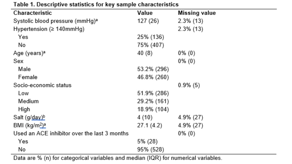
You and your colleagues have been tasked by the Kapilvastu district authorities in Nepal to help them understand the problem of high blood pressure and hypertension, and the associations between socio-demographic and health related characteristics and blood pressure level/hypertension. You have carried out a cross-sectional survey to address these aims, and collected data on systolic blood pressure, common socio-demographic characteristics, and some additional health-related characteristics. So far, you have cleaned and prepared the data. As per your statistical analysis plan you now need to compute some relevant descriptive statistics to describe the key characteristics of your sample.
Exercise 1: create a table of descriptive statistics
Aim: create a table of descriptive statistics to describe the key socio-demographic and health-related characteristics of the sample, which also describes the amount of missing data for each variable.
First, load the “SBP data final.sav” SPSS dataset. This has all the errors removed from the “SBP Excel data.xlsx” dataset we looked at last session, and all the SPSS-specific variable properties, like variable labels and value labels etc, have been updated. We will be describing the key socio-demographic and heath-related characteristics of the individuals in the dataset, who are our sample.
Next, in the “Exercises” folder also open the “Exercises.docx” Word document and scroll down to Descriptive statistics table. Your goal is to complete the empty table by calculating the values of the appropriate descriptive statistics for each of the variables in the table (i.e. the key characteristics of the sample), along with the amount of missing data for each variable, using the instructions below.
As per the footnote to the table, for each numeric characteristic/variable we will compute and present its median and then in brackets its interquartile range, e.g. if the median value was 50 and the interquartile range was 10 we would include it in the table like this: 50 (10). As for each categorical characteristic/variable we will compute the percentage and then in bracket frequency count for each category level, e.g. if the percentage of observations for a category level was 10% and the corresponding frequency count was 25 we would include it in the table like this: 10% (25). And we will also present missing data in the same way: as the percentage and in brackets the frequency count.
Note: the footnotes to the table are typical of such tables in papers and allow us to just present a single column of descriptive statistics. However, you could of course present the values in other ways, as long as it is clear what the statistics are. Once you’ve completed your table you can compare it to the completed one at the end of this section to see how you did.
Below is an explanation of the different types of descriptive statistics that are appropriate to use to describe numerical or categorical variables. Use this information to plan what types of descriptive statistics to calculate for each of the characteristics in the table, based on the type of variable that characteristic is measured by. In the dataset the variables corresponding to the characteristics in the table should be self-evident, but to avoid confusion they are (characteristic then variable name):
- Systolic blood pressure = sbp
- Hypertension = htn
- Age = age
- Sex = sex
- Socio-economic status = ses
- Salt = salt
- BMI = bmi
- Used an ACE inhibitor over the last 3 months = ace
Numerical variable descriptive statistics
- Often you will see the mean and standard deviation presented as descriptive statistics for numerical variables, but I prefer to use the median and interquartile range, so that is what we will calculate here for the numerical variables. My reason is that if the data are skewed the median is a better measure of the central tendency. However, when a variable is not skewed or not heavily skewed the mean and the median will be (often very) similar.
Categorical variable descriptive statistics
- Simply calculate the frequency (count) and the percentage (or proportion, but percentages are typically used) for each category level. E.g. for the variable sex calculate the frequency and the corresponding percentage of individuals who are male and female. This would similarly apply to a binary variable.
Present values just to 1 decimal place. We have completed the first two variables for illustration.
Calculating univariate descriptive statistics in SPSS for numerical and categorical variables
Video instructions: calculate common descriptive statistics
Written instructions: calculate common descriptive statistics
Read/hide
Calculate common descriptive statistics for categorical variables
To calculate descriptive statistics for the categorical variables we just need to produce frequency tables for each variable and extract (i.e. copy) the counts for each category level and the corresponding percentages. Simple! From the main menu go to: Analyze > Descriptive Statistics > Frequencies. Then in the Frequencies tool window add all categorical variables to the Variable(s): box. You can either drag each variable across one-by-one by clicking and holding down the left mouse button, or you can click on each one and then click the button in between the two boxes to move it over (or to move it back), or you can select multiple variables and move them at the same time in the same way by first holding down ctrl and then clicking on as many variables as you want to before moving them. Note: this is the typical behaviour of these types of variable boxes in SPSS and you will spend quite a lot of time moving variables so it’s good to try the different methods.
Once you have moved all the categorical variables in the table over to the Variable(s): box just ensure the Display frequency tables box at the bottom of the tool is ticked and then click OK. After a moment in the output window you should see the tables appear (one for each variable).
You can now copy the relevant values from the Valid Percent and Frequency columns into your Table 1 as % (n). The Valid Percent column gives the percentage for each category level after excluding any missing values, while the Percent column gives the percentage for each category level while treating any missing values as their own category level. There is no right or wrong approach but it’s more common to exclude missing data first and separately compute the % of missing values, as we do below.
Calculate common descriptive statistics for numerical variables
Now for numerical variables. Here we will be computing medians and interquartile ranges, but it’s useful to see how to check whether a variable is approximately normally distributed or skewed. There are statistical tests that can be used to formally test whether a variable’s distribution differs “significantly” from a normal distribution, but as they are based on p-value thresholds the result depends strongly on the sample size, and with a big enough sample size you are essentially guaranteed that a variable will fail the test and be classed “non-normal”. However, many statistical tests that rely on normality are quite robust to modest (or sometimes worse) departures from normality, i.e. they still work well with slightly skewed variables and have much more power than equivalent non-parametric tests. Therefore, it’s better to judge normality by eye using histograms even if this seems unscientific or less robust than using a statistical test.
So let’s see how to create histograms for numerical variables to check their distributions. In the main menu go: Graphs > Histogram. Then add the sbp variable into the Variable: box and tick the Display normal curve box just below the Variable: box. This adds a curved line to the histogram which shows what the distribution of values would look like assuming the data were normally distributed. If the histogram follows this fairly well we can assume approximate normality. Now just click OK. Do this for each numerical variable in turn and examine the graphs. What do you see? sbp, age and bmi all appear to approximate a normal distribution well, but salt displays some slight right skew.
Here won’t worry about the skew or lack of and just compute and present medians and interquartile ranges. However, if you wanted to instead present means and standard deviations (or ranges), the following approach computes them all. From the top menu go: Analyze > Descriptive Statistics > Explore. Then in the Explore tool window add each numerical variable to the Dependent List: box. Then click the Statistics button and ensure the Descriptives box is ticked and click Continue. Then back at the main Explore tool window in the Display options at the bottom ensure the Statistics option is selected and then click OK. You’ll then get several tables produced in the output window, one for each variable, with lots of descriptive statistics listed. Simply copy the relevant statistics (median and IQR) from them and add them to your Table 1 as median (IQR).
Repeat the above processes for each characteristic, given the appropriate descriptive statistic you are calculating, and complete the table.
Missing data
- To calculate the amount of missing data for each variable go Analyze > Missing Value Analysis. Then in the Missing Value Analysis tool window that appears add all variables into the Quantitative Variables: box and click OK. In the table that appears each row corresponds to one of the variables and then in the fifth column you can find the percentage of missing data and in the fourth column you can find the count of missing observations for the variable of interest. Simply copy these statistics into your Table 1’s “Missing value” column for each corresponding variable as % (n).
Example completed table for reference
Read/hide
If you have any glaring errors or strange differences try and work out why, and if you can’t then ask for help!