The independent t-test
In this practical we will practice applying the independent t-test to analyse the association between a normally distributed numerical outcome and a binary covariate, or put in more real-world terms: whether and by how much the mean of a numerical outcome differs between two groups.
Rationale
The independent t-test allows you to compare whether two independent groups differ in their mean values for a numerical outcome, assuming that the values of the outcome are approximately normally distributed in each group (although it’s quite robust even if the outcome values are pretty non-normally distributed in each group). The term “independent t-test” can often be used just to refer to a hypothesis test, and therefore effectively just a p-value, but we will focus on using it (or more broadly the t-distribution) to estimate the mean difference in a numerical outcome between two groups and the confidence intervals around that mean difference, because as you hopefully now appreciate that tells us so much more about the likely direction and size/magnitude of the association of interest in the target population than just a p-value!
For example, if you wanted to analyse whether a group of women had a different mean systolic blood pressure from a group of men. Note: with the independent t-test the covariate is binary and might naturally consist of a categorical variable with just two levels (like sex if there are just the levels female and male). Or we might construct a binary variable from a categorical variable with >2 levels (e.g. reclassifying socio-economic status from low, medium and high levels to just low/medium and high levels by pooling individuals in the low and medium levels). Or we might create a binary variable from a numerical variable based on a threshold cut-off (e.g. BMI ≤20 vs BMI >20). We’ll look at the last of these scenarios as it requires a bit more preparation, so you will know how to do this if needed in SPSS.
Practice
Scenario
You and your colleagues have been tasked by the Kapilvastu district authorities in Nepal to help them understand the problem of high blood pressure and hypertension, and the associations between socio-demographic and health related characteristics and blood pressure level/hypertension. You have carried out a cross-sectional survey to address these aims, and collected data on systolic blood pressure, common socio-demographic characteristics, and some additional health-related characteristics. As per your statistical analysis plan you need to explore the association between important characteristics and levels of systolic blood pressure. These are therefore descriptive research questions, as we do not assume any causal association are necessarily behind any observed association, and the aim of these analyses is to help policy makers target preventative efforts at the most at-risk groups, as identified by their key characteristics.
Below we will just look at one of these associations. Specifically, the association between age, when grouped as individuals <=40 and individuals >40, and the level of systolic blood pressure in mmHg.
Exercise 1: use the independent t-test to analyse how the mean level of systolic blood pressure (mmHg) differs between individuals <=40 and >40
Step 1: create a binary covariate from a numerical variable
Of course you may be interested in the association between a numerical covariate that is already binary, e.g. sex with levels of female and male, but this is a good opportunity to see how we can get SPSS to convert a numerical variable into a binary variable based on a threshold cut-point.
- Load the “SBP data final.sav” SPSS dataset.
Video instructions: create a binary covariate from a numerical variable
Written instructions: create a binary covariate from a numerical variable
Read/hide
Next we need to create a two-level categorical variable defining our younger and older individuals. Usually you should choose the cut-point at which you define your two-levels based on theory or some sensible motivation (e.g. the age at which prior research suggests blood pressure may often change), but here let’s just compare those individuals above and below the median age, which is 40. We therefore want to create a variable that classifies every individual as either ≤40 or >40.
- First, we can use the Compute Variable tool to create a new variable based on a logical test of whether the value in the original age variable is ≤40 or not. This will create a new variable that has the value 0 if the participant’s age is >40 and the value 1 if their age is ≤40 (i.e. if the logical check we asked SPSS to do on the original age variable is TRUE then the new variable’s value is 1). From the main menu go: Transform > Compute Variable. Then in the Compute Variable tool enter “age_young_old” as the name for the new variable in the Target Variable: box. Then in the Numeric Expression: box enter:
age <= 40
Then click OK.
The output window will appear. Minimise this to go back to the main window and go to the Variable View. You should now see our new variable age_young_old has appeared. Let’s give it a variable label so it’s well described in SPSS: Age (0 = >40 / 1 = <=40). Then let’s give it some value labels so each level is well described. As it was created from a logical expression it takes only two values: 0 or 1. 1 should be coded as “≤40”, because when the participant’s age was less than or equal to 40 the logical expression would be true and the new variable would take the value 1. Similarly 0 should be coded as “>40” as the logical expression would be false and the value set to 0. Check back to the instructions on adding value labels or ask if you need help.
Lastly, once that’s done you should always do a quick check that the variable has been created correctly using a “cross tabulation” between our old and new age variable. In the main menu go: Analyse > Descriptive Statistics > Crosstabs. Then in the Crosstabs tool add the original age variable into the Row(s): box and the new categorical binary age variable into the Column(s): box and click OK. If you’ve created the new age variable correctly all ages ≤40 should be counted in the age <=40 column and all ages >40 in the new age variable age >40 column. Always perform such checks when creating new variables!
Step 2: check the assumptions of the independent t-test are not violated
Read/hide
Whenever you run a statistical analysis you must ensure that the assumptions of the analysis are not violated, otherwise the results may not be valid or even meaningful. For simple analyses like the independent t-test we can check the assumptions before we run the test, but for more sophisticated analyses such as regression models we typically check the assumptions after running the analysis because SPSS produces the information to make the necessary checks only after running the analysis.
The independent t-test makes the following assumptions:
1. Continuous outcome
Technically an independent t-test assumes a continuous outcome variable, but as long as assumptions 2 and 3 below are satisfied it’s fine to use a discrete outcome with an independent t-test. Here our outcome is continuous. Note: ideally when analysing a discrete outcome you would use a more specific model like a Poisson or negative binomial model, but this is beyond the scope of this introductory course.
2. Independent groups (hence the “independent t-test”)
This means the observations in each group cannot be related. You can only really verify this by knowledge of your study design. With the SBP data the study took a simple random sample of individuals and we are then dividing them into two groups based on an age threshold. Therefore, by definition the two groups are statistically independent as all observations represent separate, randomly sampled individuals.
Typically groups are only not independent in two situations. First, if you were taking repeated measurements from the same set of individuals but treating the measurements at each time period as different “groups”. Here there would be correlations between the measurements at the different time periods within individuals. Second, if you were taking measurements from two groups of separate individuals, but the individuals in the two groups were not statistically independent. For example, if there were different families with members in both the age groups, or if there were individuals from the same work places within each group. Again, in such situations there would be correlations between members of the same family or work place (e.g. due to genetics or shared risk factors etc).
Here our groups or observations are clearly independent as the individuals in the study were randomly sampled and the two groups contain separate individuals.
3. The outcome is approximately normally distributed within each group
Note: technically it is the “residuals” or “model errors” that need to be normally distributed, which are the differences between the observed values of the data and the “model predicted values”. For a t-test these are simply the differences between the observed values of the data and the mean of the relevant group that the observation comes from, which actually means that for a t-test the residuals are identical to the observed values and so you can just view the distribution of the observed data. For more complicated regression models we’ll see that we need to calculate and plot the residuals separately.
To check the distribution of the residuals within each group you can use statistical tests, but most statisticians would recommend using graphical methods. We can visually check these two distributions easily in SPSS using histograms as follows. From the main menu go: Graphs > Histogram. Then add the sbp variable into the Variable: box, then add the age_young_old variable into the Rows: box, tick the Display normal curve box and then click OK. You’ll see a histogram for the sbp variable for each age group. As you can see the outcome approximates a normal distribution fairly well for the ≤40 age (this is probably as good as you would see with real data), and is slightly right skewed for the >40 age group. However, as previously mentioned the t-test is pretty robust to slightly skewed outcomes so this is nothing to worry about, and we can assume this assumption is met. Below are some examples of suitably and unsuitably distributed data for you to compare with for future reference.
Examples of suitably and unsuitably distributed data for t-tests
Read/hide
Students (and researchers) often struggle with knowing whether an analysis’s assumptions have been violated or not, and for good reason because it usually involves judgement based on experience. For the t-test like most analyses requiring normality there is no agreed “threshold” for when the skewness of a variable is considered “non-normal”. However, as t-tests and regression models are fairly robust to some non-normality the following examples should hopefully give you a sense of when you are okay to go ahead and when you are violating the assumptions and need to transform the data or use a different model.
A. Probably suitably approximately normally distributed data within each group for a t-test, with n = 50 per group:
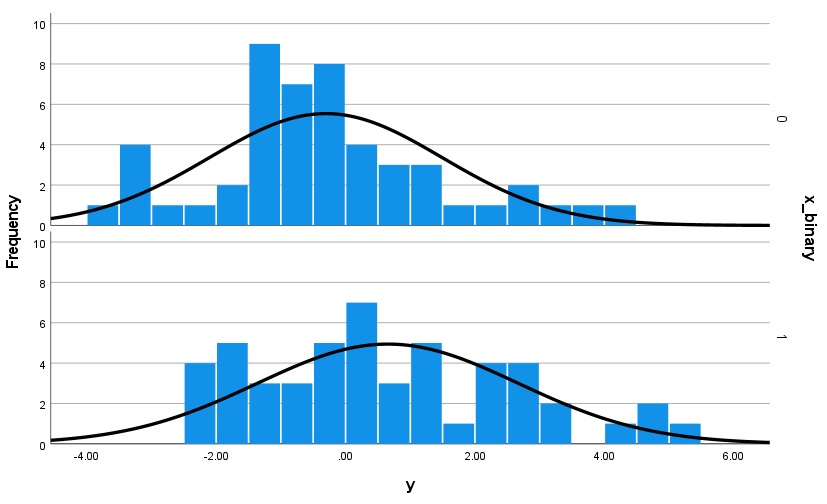
With only 50 data points per group the distribution is pretty “lumpy” but you can see an approximate normal distribution in both groups, although less so for the lower group. Also note: these data are generated from a normal distribution, so you can see that when your sample size is low even with artificially simulated data from a known normal distribution the resulting sample can often be only somewhat approximately normal! You can also see that the variance in both groups looks approximately normal, which satisfies our next assumption (see below).
B. Highly suitably normally distributed data within each group for a t-test, with n = 500 per group:
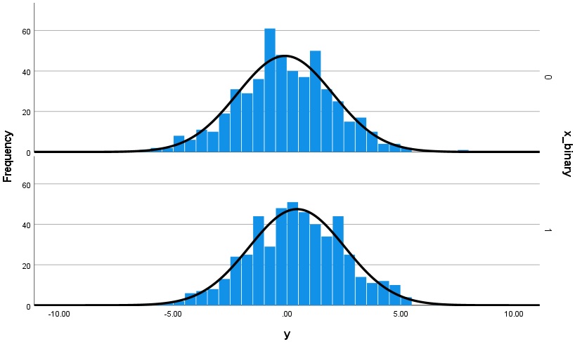
Now with 500 data points per group simulated from the same distribution unsurprisingly the distribution looks much more suitably normal.
C. Probably not suitably normally distributed data within each group for a t-test, with n = 50 per group:
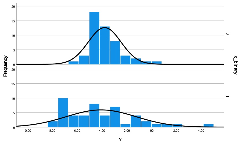
You may think it doesn’t look much different from the first image, and you’d be right. Again, it comes down to judgement but when sample sizes are small there’s a lot of subjectivity involved. These data are simulated from a right-skewed “version” of the normal distribution. If you are concerned one option is to run your test on the raw data and then transform the data (we’ll see later how to do this) and re-run the test and see if the results change much, and just report both. This is called a sensitivity analysis.
You can also see that there is a lot more variance in the lower group’s data, which would violate our next assumption (see below).
D. Definitely not suitably normally distributed data within each group for a t-test, with n = 500 per group:
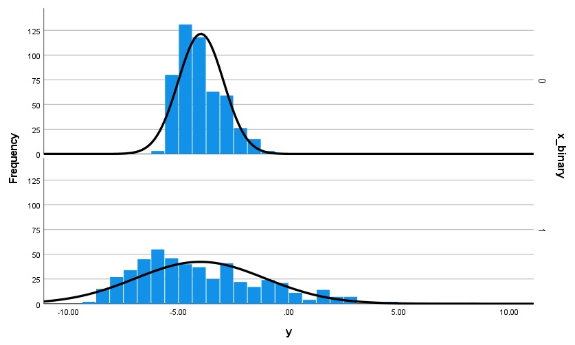
Now with 500 observations per group it’s clear that there is some definite right-skew in the distribution of both group’s data, and that there is considerably more variance in the lower group.
4. Equal variances in each group
This means that the variance (dispersion or spread) of outcome values is approximately the same in each group. We can check this by looking at the p-value for a test of this assumption called “Levene’s test of equality of variances” or by comparing the histograms from the two groups. SPSS produces the results of the Levene’s test when we run the t-test, so we will evaluate the results of this test/assumption once we’ve produced our t-test results below. Note: if this test is significant (P<0.05) we can simply use the results from the version of the t-test that doesn’t assume equal variances in each group. The only disadvantage is that we lose a little bit of statistical power, but typically it’s not much and the results will be very similar. Hence, although we’ll interpret the “equal variances assumed” version of the t-test below it’s probably a better practice to just always use the more conservative but robust and safer set of results that do not assume equal variances is each group.
Step 3: run the independent t-test
Video instruction: run the independent t-test
Written instruction: run the independent t-test
Read/hide
In the main menu go: Analyse > Compare Means > Independent Samples T Test. Then in the Independent-Samples T Test tool add the sbp variable into the Test Variable(s): box. Then add our new covariate for age group (at the bottom of the list) into the Grouping Variable: box and click Define Groups…. This is where we tell SPSS what numerical values code for each of our two groups, and what way round we want to compare the two groups. Remember we created the age variable so that it took the value “0” for individuals >40 and “1” for individuals ≤40. Let’s compare individuals >40 to individuals ≤40. When it comes to comparing the groups this tells SPSS subtract the mean outcome in group 0 from group 1, i.e. the mean systolic blood pressure for individuals >40 minus the mean systolic blood pressure for individuals ≤40. To do this ensure the Use specified values option is selected and add the value “0” to Group 1: and the value “1” to Group 2:.
Note: you can of course swap the coding values around and compare individuals ≤40 to individuals >40 and your results will be reversed but otherwise identical. Neither choice is necessarily “correct” it just depends on which way round you want the groups compared. If, in your version of SPSS, there is a box called Estimate effect sizes below the Grouping variable: options make sure this is not ticked. Finally click Continue and then OK. You’ll now see the output window appear with our results!
Step 4: understand the results tables and extract the key results
Now we’ve verified the first two assumptions of the independent t-test (independent observations and approximately normally distributed residuals) let’s look at the results tables where we can check the third assumption (equal variances in each group), extract the key results and interpret them.
So what do the tables mean?
Group Statistics table explained
The first table we see gives us descriptive statistics for the outcome variable for each level of our categorical covariate.
First, make sure you look at and record the values under the “N” column, which are the group sample sizes, and check they match what they should be. You should see there were 295 individuals in the ≤40 group and 248 individuals in the >40 age group. These sum to 543, which is less than the total number of individuals in the dataset: 556. There are three reasons why this might be: either some individuals are missing values for the outcome or the covariate or both variables. We know from when we prepared the dataset that some individuals are indeed missing values for their systolic blood pressure. You can quickly check this by going to the Data view, right clicking on the sbp variable and selecting Descriptive Statistics. In the Statistics results table that appears you should see that there are indeed 13 individuals with missing values for sbp, and hence only 543 individuals with complete data on this variable, which explains the sample size of the independent t-test.
Next make sure you look at and record the mean value of the outcome for each group under the “Mean” column. You should see the mean systolic blood pressure (mmHg) was 128.2 for individuals >40 and 125.1 for individuals ≤40 (rounded to 1 decimal place).
Independent Samples Test
This table gives us the results of the t-test we’re interested in, although SPSS lays out the results less than clearly in my opinion. Here’s what they all mean.
Levene’s Test for Equality of Variances section columns explained
Under this part of the table are results that relate to a statistical test that is totally separate to the independent t-test called “Levene’s test for equality of variances”. This tests whether the variance (spread) of the outcome in each group is approximately equal. If they are not then this assumption is violated and we must only use the results from the version of the independent t-test that accounts for this.
F
- The F-value is the test statistic for the Levene’s test for equality of variances. You can ignore it as it is used to calculate the corresponding p-value of the test (see below), which is all we are interested in.
Sig.
The “Sig.” value is just the p-value associated with the test statistic (i.e. the F-value). For some reason SPSS always refers to p-values with a “Sig.” column heading. The null hypothesis for the Levene’s test is that the variances in both groups are equal. Therefore, if the p-value (“Sig.”) is <0.05 this indicates that the variances in the two groups are unlikely to be equal. If this is the case it is then safer to use the version of the independent t-test that does not assume equal variances. Results from both versions of the independent t-test are presented. Just look at the far left of the table and you can see the top row of results are for the “Equal variances assumed” version and the bottom row for the “Equal variances not assumed” version.
Here you should see that the p-value for the test is 0.244, i.e. it’s >0.05. Therefore, we can assume the variances are approximately equal in each group. Hence, we can use the results for the independent t-test from the row called Equal variances assumed (see below).
Note: SPSS only gives p-values to 3 decimal places, so when it says “0.001” it means the p-value is actually <0.001. Therefore, you should write P<0.001.
t-test for Equality of Means section columns explained
Under this part of the table are the results for the actual independent t-test. We will use those from the row/version that do not assume equal variances.
t
- This is the value of the t-test statistic which is used when calculating the p-value. We can ignore this and just interpret the p-value directly (and of more use the confidence intervals).
df
- This is the degrees of freedom which form part of the calculation of the test statistic (calculated as: n - 2). You can typically ignore this but it should closely match your “true” sample size, i.e. the number of genuinely independent observations.
Sig. (2-tailed)
This is the two-tailed p-value for the independent t-test. The “two-tailed” part means that it allows for the possibility that the difference between the two groups may be positive or negative, i.e. either group might have a greater mean than the other. The null hypothesis of the independent t-test is that the “true” difference between the two groups in the target population from which the sample was taken is exactly 0. Therefore, this p-value tells us how likely we are to have observed data giving a mean difference at least as great or greater (in either direction) as the one observed. Alternatively, you can more loosely interpret it as a probability measure of how consistent the data are with the null hypothesis of no difference. Again note that SPSS only gives p-values to 3 decimal places, so when it says 0.001 it means the p-value is <0.001.
Here you should see that the p-value is 0.072.
Mean Difference
This is the difference between the mean of the outcome for the group that we set as “Group 1” minus the mean of the outcome for “Group 2”. For us this means the mean SBP of participants aged >40 minus the mean SBP of those aged ≤40. It therefore tells us the direction and size of any difference, and is therefore a key result/statistic from the test. You can swap the coding of the groups around if it makes more sense (just go back and re-run the analysis but change the coding), but the difference will be reversed (i.e. a positive difference will become a negative difference).
Here you should see that the mean difference (rounded to one decimal place) is 3.1.
Std. Error Difference
- This is the standard error of the mean difference, which estimates the sampling variability associated with our estimate of the parameter in the target population. This is used when calculating the 95% confidence intervals and the p-value. You can ignore it and just interpret the confidence intervals and p-value.
95% Confidence Interval of the Difference (Lower and Upper)
These are the estimated lower and upper 95% confidence intervals around the estimated mean difference, which is the point estimate or best single estimate of the mean difference in the target population. Formally speaking, if we repeated our study an infinite (or very large number) of times and each time we calculated the mean difference and the 95% confidence interval around those mean differences then 95% of those 95% confidence intervals would contain the true mean difference found in the target population (i.e. the mean difference that we would find if we sampled 100% of the target population). Informally speaking we can think of the 95% confidence intervals as defining a range of values that are consistent with the likely/probable true mean difference in the target population based on the sampled data.
Here you should see that the lower and upper confidence intervals for the mean difference (rounded to one decimal place) are -0.3 and 6.4.
Step 5: report and interpret the results
Reporting the results
In a methods section you should explain that you used an independent t-test to analyse the data and justify why.
In a results section we would want to report the sample size, the mean of the outcome for each group, and the key results of the independent t-test (the mean difference, the 95% confidence intervals and the associated p-value). Therefore, we could write something like the following (using “n” as it is commonly used to refer to sample size):
We compared the systolic blood pressure among individuals aged >40 (n = 248) to those aged (n = 295). Among those aged >40 the mean systolic blood pressure was 128.2 mmHg and among those aged ≤40 the mean systolic blood pressure was 125.1 mmHg. Using an independent t-test (equal variances assumed) we estimated that the mean difference in systolic blood pressure between those aged >40 compared to those aged ≤40 was 3.1 mmHg (95% CI: -0.3, 6.4).
Note: the convention is to compactly present confidence intervals for estimated statistics in brackets like above, indicating the confidence level of the confidence interval (usually 95%), and to use a comma “,” or possibly the word “and” to separate the lower and upper confidence interval, but not a dash “-” as this can look like a negative symbol.
Also note: we are focusing on the mean difference and the confidence intervals, not the p-value here as it tells us nothing more and far less than those results do.
Lastly, if you felt it wasn’t clear where the inferential result had come from, say if you were reporting result from different analyses, then you should certainly make this clear in the results section too, e.g. you might say something like “based on an independent t-test the mean difference was…”.
Discussion: interpret the direction and size of the difference in terms of the implications for practice and policy. Is the difference “statistically significant”, i.e. can we make a clear inference that there even is a difference on average between the groups, and if so is it a small difference, a medium difference, a large difference etc in terms of what is being measured and the implications for practice and policy?
Interpreting the results
How do we actually interpret these results then? Remember with statistical inference we are aiming to make a “probabilistic inference”, or a generalisation with some level of uncertainty, about the likely value of the population parameter of interest, which here is the mean difference in systolic blood pressure between individuals aged >40 compared to individuals aged ≤40 in our target population, based on the data from our sample. And our confidence intervals around our sample statistic (the sample mean difference) are what allow us to do that. More specifically, the confidence intervals around the mean difference tell us that the mean difference in systolic blood pressure between individuals aged >40 compared to individuals aged ≤40 in the target population is “quite likely” to be somewhere between -0.3 and 6.5 mmHg. Alternatively and equivalently we can interpret the results in terms of a randomly selected individual in our target population, and say that if we randomly selected one individual from the <=40 group and one from the >40 group then on average the systolic blood pressure of the individual in the >40 would be “quite likely” to be between -0.3 mmHg lower to 6.5 mmHg higher than the individual in the ≤40 group.
Note: strictly or technically speaking our confidence intervals tell us how much error is associated with our sampling process, and that if we repeated our study many times 95% of the time the 95% confidence intervals that we obtained around our estimated mean difference would contain the true mean difference in the target population. Therefore, our interpretation of the value being “quite likely” to fall within our given confidence interval range is somewhat informal and loose.
Also note: critically this interpretation assumes that all other sources of bias are negligible, which is extremely unlikely! Therefore, you should always treat inferential results very carefully, and evaluate them in the context of how much likely bias there is in the results other than sampling error, which is the only source of bias that inferential statistics account for. E.g. if you knew there was likely a large amount of other sources of error in the study, such as some serious selection bias, then the 95% confidence intervals would not accurately reflect the total error or bias in the results because they can only account for sampling error in the absence of all other errors/bias.
Consequently, our confidence intervals indicate that we can’t have much confidence over whether there is even a positive or negative difference in systolic blood pressure between these two groups in the target population, let alone how big any difference is with any great precision. However, the result does tell us that the practical significance or clinical significance of the true difference in mean systolic blood pressure between these two groups is likely to be small, given the confidence intervals suggest it is likely to be at most just 6.5 mmHg (the confidence interval furthest from 0). Always remember though, this is a probabilistic result (not certain) and there is always still a non-negligible chance that the true difference is greater, possibly much greater, than we estimated, i.e. outside the range of the 95% confidence intervals, and as above this is actually inevitable with any study unless completely free of other sources of bias.
Lastly, note: when setting up the t-test if we swapped the order of the comparison around we would get the same result but expressed as the ≤40 age group compared to the >40 age group, and so we’d get a mean difference of -3.1 mmHg (95% CI: -6.5, 0.3). Note the 95% confidence interval order is also reversed.
Exercise 2: use the independent t-test to analyse how the mean level of systolic blood pressure (mmHg) differs between individuals with BMI <30 kg/m² and ≥30 kg/m²
Using the “SBP final data.sav” dataset and via the process outlined above use an independent t-test to analyse the association between BMI and systolic blood pressure.
Divide bmi into two groups based on BMI values <30 kg/m² and those ≥30 kg/m², which are the values typically used to define obesity when defined in terms of BMI.
Compare individuals with BMI values <30 kg/m² to those with BMI values ≥30 kg/m² using the independent t-test.
Extract the mean difference and confidence intervals around this estimate.
In the “Exercises” folder open the “Exercises.docx” Word document and scroll down to Independent t-test: the association between BMI and systolic blood pressure.
Write a couple of sentences reporting the results of your analysis. Include the basic descriptive statistics: sample size, group sizes and group outcome means. Also be sure to include sufficient details about the outcome variable and the comparison made, including how the two independent groups were defined, as well as the type of analysis used, and of course the key inferential results. Round results to one decimal place. You don’t need to explain anything about the study or interpret the clinical or practical importance of the result.
Write a sentence or two about the key limitations of this analysis in terms of interpreting the result.
Once you’ve completed this compare your reporting to the below example text.
Example independent t-test results reporting text
Read/hide
Using an independent t-test I analysed the association between BMI and systolic blood pressure (mmHg) for individuals having low compared to high BMI (<30 kg/m² compared to ≥30 kg/m²). Out of a total sample size of 516 individuals, 419 individuals had a BMI <30 kg/m² (mean systolic blood pressure = 121.6 mmHg) and 97 individuals had a BMI ≥30 kg/m² (mean systolic blood pressure = 146.7 mmHg). This represented a mean difference of -25 mmHg (95% CI: -28.9, -21.2) for those with a BMI <30 kg/m² compared to those with a BMI ≥30 kg/m². Therefore, having a BMI < 30 kg/m² appears to be associated with a substantially lower systolic blood pressure on average than having a BMI ≥30 kg/m².
Next steps (optional)
If you have time and want to practice and learn more you can try the following exercises:
Repeat the independent t-test but reverse the coding of the groups to convince yourself that the results are identical but just reversed.
Use the independent t-test to analyse whether there is a difference in the mean systolic blood pressure between individuals from different socio-economic groups (ses variable). As there are three socioeconomic groups in the variable this would require you to first recode the ses variable into a new variable so that two of the socio-economic groups are pooled to give a binary variable.